The Small Perturbation Method for 2D scattering from Gaussian random rough surface
Contents
- The scattering amplitude
- The perturbative expansion
- The Dirichlet boundary condition
- The Neumann boundary condition
- The transmission problem for S-polarized electromagnetic waves
- The transmission problem for P-polarized electromagnetic waves
- Stationary random rough surface with normal height distribution and Gaussian roughness spectrum
- *** THE COHERENT REFLEXION COEFFICIENT ***
- The Dirichlet boundary condition
- The incoherent bistatic coefficient
- *** THE DIFFERENTIAL REFLECTIVITY ***
- Monostatic diagrams
- Bistatic diagrams
- Summary - 2D scattering
The scattering amplitude
For an incident plane wave impinging from air a  -invariant surface
  with an angle
  from the
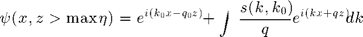
  -axis, the field in the air above the surface region (that is
  writes as the plane wave sum :
 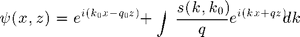 for an implicit
  time dependency. With wavenumber
  ,
,  and
and  define the incident wavevector. For the scattering one,
  is chosen so that
  with
with  .
.
lambda=1;       % the EM wavelength is chosen as length unit
K0=2*pi/lambda;
qf=@(k,ep) sqrt(K0^2*ep-k.^2); % ep=1 in air
The perturbative expansion
Assuming  and following the small perturbation method (SPM), the scattering amplitude
  is expanded into a series :
  where
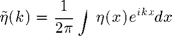
where  is the Fourier transform of the height function
 and the coefficients
  are roughness-independent.
The Dirichlet boundary condition
Enforcing  on the surface leads to :

 with
with 
BD0=@(k0) -qf(k0,1);
BD1=@(k,k0) 2*1i*qf(k,1).*qf(k0,1);
BD2=@(k,x,k0) 2*qf(k,1).*qf(x,1).*qf(k0,1);
The Neumann boundary condition
Enforcing  on the surface leads to :


BN0=@(k0) +qf(k0,1);
BN1=@(k,k0) -2*1i*(K0^2-k.*k0);
BN2=@(k,x,k0) -2*(K0^2-k.*x).*(K0^2-k0.*x)./qf(x,1);
The transmission problem for S-polarized electromagnetic waves
Assuming continuity of both the field  and its normal derivative
  when passing from air (wavenumber K_0) to the scattering medium (wavenumber
  ), we first define reflection
  coefficient for the plane :
 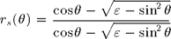 and associated transmission coefficient
 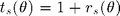 . Then,

This corresponds to the transmission problem of an electromagnetic wave which electric field is parallel to the invariance direction , between air and a nonmagnetic medium of relative permittivity  .
.
rs=@(k,ep) (qf(k,1)-qf(k,ep))./(qf(k,1)+qf(k,ep));
ts=@(k,ep) 1+rs(k,ep);
BS0=@(k0,ep) +qf(k0,1).*rs(k0,ep);
BS1=@(k,k0,ep) 0.5*1i*K0^2*(ep-1).*ts(k,ep).*ts(k0,ep);
The transmission problem for P-polarized electromagnetic waves
Now considering an electromagnetic wave wich electric field is in the incidence plane, that is perpendicular to the invariance direction , it is the quantity  that is continuous besides filed . When passing from air (wavenumber K_0) to the scattering medium (wavenumber ), we first define reflection
  coefficient for the plane :
 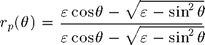 and associated transmission coefficient
  . Then,

This corresponds to the transmission problem of an electromagnetic wave which electric field is parallel to the invariance direction , between air and a nonmagnetic medium of relative permittivity .
rp=@(k,ep) (ep*qf(k,1)-qf(k,ep))./(ep*qf(k,1)+qf(k,ep));
tp=@(k,ep) 1+rp(k,ep);
BP0=@(k0,ep) +qf(k0,1).*rp(k0,ep);
BP1=@(k,k0,ep) 0.5*1i*((ep-1)*(ep*k.*k0-qf(k,ep).*qf(k0,ep))/ep^2).*tp(k,ep).*tp(k0,ep);
Stationary random rough surface with normal height distribution and Gaussian roughness spectrum
The surface is a stationary centered random process with normally-distributed height. The roughess spectrum  , Fourier transform of the two-points correlation function
  , with brackets denoting statistical averaging, is a Gaussian function with two parameters
  and
and  the height root mean quare and correlation length, respectively.
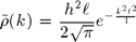
h=lambda/50;
l=lambda/2;
spec=@(k) (0.5*h^2*l/sqrt(pi))*exp(-0.25*k.^2*l^2);
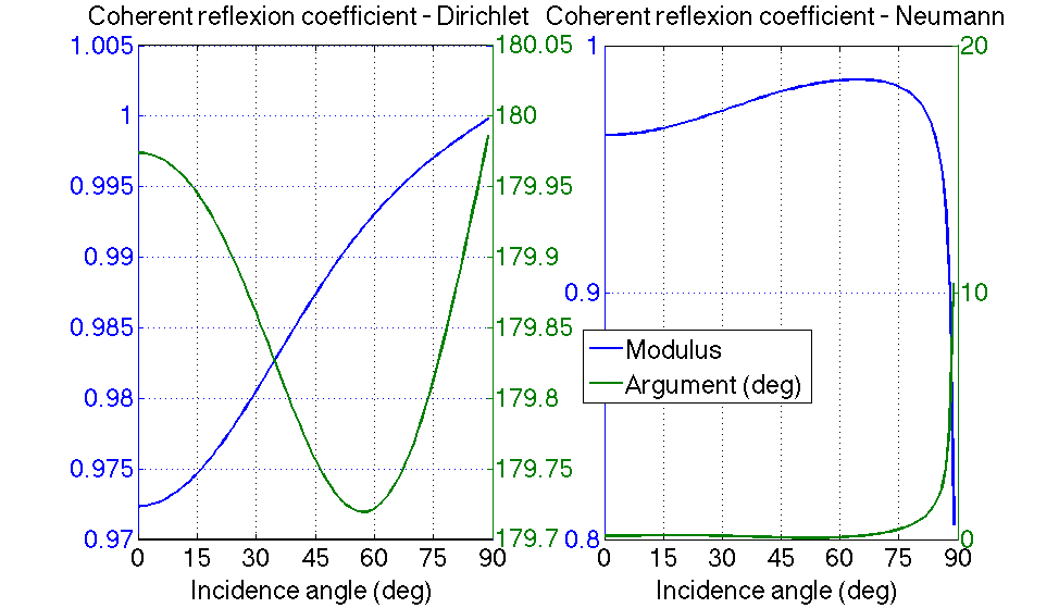
*** THE COHERENT REFLEXION COEFFICIENT ***
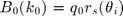
Stationarity implies that the mean field writes in air above the surface region :  as the sum of the incident field and a specularly-reflected plane wave. The amplitude of that reflection defines the coherent reflexion coefficient. It is related to the scattering amplitude by :
 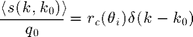 in the general case, and applying the third-order SPM expansion to Gaussian process,
  since, due to the Gaussian moment theorem, first- and third-orders do not contribute.
xmax=6*(sqrt(2)/l); % integration bound for Gaussian spectrum
rc=@(k0,B0,B2) B0(k0)./qf(k0,1)+integral(@(x)B2(k0,k0+x,k0).*spec(x)./qf(k0,1),-xmax,xmax);
The Dirichlet boundary condition
tid=[0:35 37:89];
for ii=1:length(tid)
    spm2rcd(ii)=rc(K0*sind(tid(ii)),BD0,BD2);
    spm2rcn(ii)=rc(K0*sind(tid(ii)),BN0,BN2);
end
figure(1)
subplot(121)
[AX,H1,H2]=plotyy(tid,abs(spm2rcd),tid,angle(spm2rcd)*180/pi);grid on
set(AX(1),'FontSize',24,'XLim',[0 90],'XTick',[0:15:90])
set(AX(2),'FontSize',24,'XLim',[0 90],'XTick',[0:15:90])
set(H1,'LineWidth',2)
set(H2,'LineWidth',2)
xlabel('Incidence angle (deg)')
title('Coherent reflexion coefficient - Dirichlet')
subplot(122)
[AX,H1,H2]=plotyy(tid,abs(spm2rcn),tid,angle(spm2rcn)*180/pi);grid on
set(AX(1),'FontSize',24,'XLim',[0 90],'XTick',[0:15:90])
set(AX(2),'FontSize',24,'XLim',[0 90],'XTick',[0:15:90])
set(H1,'LineWidth',2)
set(H2,'LineWidth',2)
xlabel('Incidence angle (deg)')
title('Coherent reflexion coefficient - Neumann')
legend('Modulus','Argument (deg)','Location','Best')
The incoherent bistatic coefficient
With  the incoherent scattered amplitude, the incoherent bistatic coefficent
  is defined by
  For a Gaussian process, the SPM expansion leads to :
  since, due to the Gaussian moment theorem, the third-order contribution vanishes.
*** THE DIFFERENTIAL REFLECTIVITY ***
In air, the time-averaged power density through an horizontal plane is proportional to 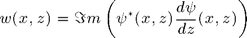 It writes
  for the incident plane wave and
  for the statistically averaged scattered field. Note that only the propagative part of the scattered field contributes. The reflectivity
 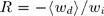 thus writes :
 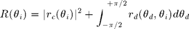 introducing
  the (incoherent) differential reflectivity :
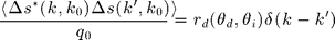
rd=@(k,k0,B1) abs(B1(k,k0)).^2.*spec(k-k0)./qf(k0,1);
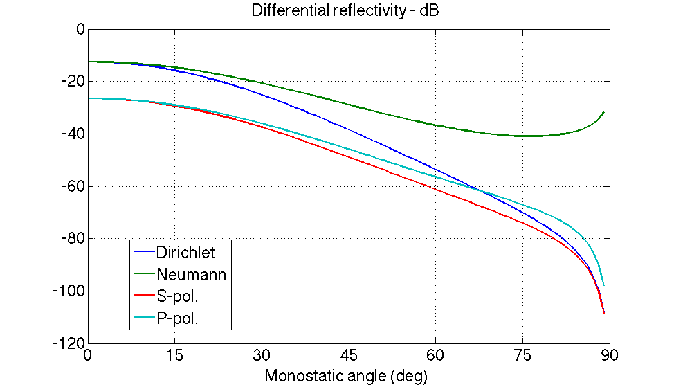
Monostatic diagrams
tid=[0:89];
k0=K0*sind(tid);
k=-k0; % backscattering configuration
spm1rdd=rd(k,k0,BD1); % Dirichlet
spm1rdn=rd(k,k0,BN1); % Neumann
ep=2.25; % dielectric constant of glass at optical frequencies
spm1rds=rd(k,k0,@(k,k0)BS1(k,k0,ep)); % S-pol.
spm1rdp=rd(k,k0,@(k,k0)BP1(k,k0,ep)); % P-pol.
dB=@(x) 10*log10(x);
figure(2)
H1=plot(tid,dB(spm1rdd),tid,dB(spm1rdn),tid,dB(spm1rds),tid,dB(spm1rdp));grid on
set(gca,'FontSize',24,'XLim',[0 90],'XTick',[0:15:90])
set(H1,'LineWidth',2)
xlabel('Monostatic angle (deg)')
title('Differential reflectivity - dB')
legend('Dirichlet','Neumann','S-pol.','P-pol.','Location','Best')
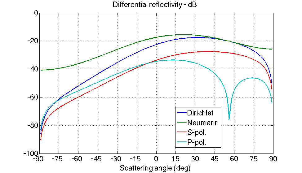
Bistatic diagrams
ep=2.25; % dielectric constant of glass at optical frequencies
tid=atand(sqrt(ep)); % The BREWSTER angle
fprintf('The Brewster angle is %gdeg for index %g\n',tid,sqrt(ep))
k0=K0*sind(tid);
tsd=[-89:89];
k =K0*sind(tsd);
spm1rdd=rd(k,k0,BD1); % Dirichlet
spm1rdn=rd(k,k0,BN1); % Neumann
spm1rds=rd(k,k0,@(k,k0)BS1(k,k0,ep)); % S-pol.
spm1rdp=rd(k,k0,@(k,k0)BP1(k,k0,ep)); % P-pol.
dB=@(x) 10*log10(x);
figure(3)
H1=plot(tsd,dB(spm1rdd),tsd,dB(spm1rdn),tsd,dB(spm1rds),tsd,dB(spm1rdp));grid on
set(gca,'FontSize',24,'XLim',[-90 90],'XTick',[-90:15:90])
set(H1,'LineWidth',2)
xlabel('Scattering angle (deg)')
title('Differential reflectivity - dB')
legend('Dirichlet','Neumann','S-pol.','P-pol.','Location','Best')
The Brewster angle is 56.3099deg for index 1.5
Summary - 2D scattering
The rough surface reflectivity decomposes as with  the coherent reflexion coefficient and
  the (incoherent) differential reflectivity both obtained from the scattering amplitude , itself defined through