The 1st-order SPM for 2D scattering a from deterministic rough surface

The scattering amplitude
The perturbative expansion
Load the rough surface profile
The Dirichlet boundary condition
The Neumann boundary condition
The transmission problem for S-polarized electromagnetic waves
The transmission problem for P-polarized electromagnetic waves

The scattering amplitude

For an incident plane wave impinging from air a $y$ -invariant surface $z=\eta(x)$ with an angle $\theta_i$ from the $z$ -axis, the field in the air above the surface region (that is $z>\max\eta)$ writes as the plane wave sum : 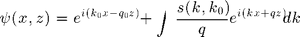$\psi(x,z)=e^{i(k_0x-q_0z)}+\int\frac{s(k,k_0)}{q}e^{i(kx+qz)}dk$ for an implicit $e^{-i\omega t}$ time dependency. With wavenumber $K_0=\frac{\omega}{c}=\frac{2\pi}{\lambda}$ , $k_0=K_0\sin\theta_i$ and $q_0=K_0\cos\theta_i$ define the incident wavevector. For the scattering one, $q$ is chosen so that $k^2+q^2=K_0^2$ with $0\le\arg q\le\pi/2$ .

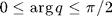lambda=1;                   % the EM wavelength is chosen as length unit
rL=64*lambda;               % length of the surface
N=20*rL;                    % number of sampling points
kx=[-N/2:N/2-1]'*2*pi/rL;   % spatial frequencies
tid=[-89:89];               % incidence angles
tsd=[-89:89];               % scattering angles
K0=2*pi/lambda;             % EM wavenumber
qf=@(k,ep) sqrt(K0^2*ep-k.^2); % ep=1 in air

The perturbative expansion

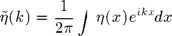
Assuming $\epsilon=\eta/\lambda\ll 1$ and following the small perturbation method (SPM), the scattering amplitude $s(k,k_0)$ is expanded into a series : $s(k,k_0)=B_0(k_0)\delta(k-k_0)+B_1(k,k_0)\tilde\eta(k-k_0)+\int B_2(k,x,k_0) \tilde\eta(k-x)\tilde\eta(x-k_0)dx+\int B_3(k,x,y,k_0) \tilde\eta(k-x)\tilde\eta(x-y)\tilde\eta(y-k_0)dxdy+O(\epsilon^4)$ where $\tilde\eta$ is the Fourier transform of the height function $\eta$ $\tilde\eta(k)=\frac{1}{2\pi}\int\eta(x) e^{ikx}dx$ and the coefficients $B_n$ are roughness-independent.

tfdir=@(z) fftshift(fft(fftshift(z)))*(rL/N)/(2*pi);    % Fourier transform of the surface profile
spm=@(B1,z,k,k0) B1(k,k0).*interp1(kx,tfdir(z),k-k0);   % 1st-order SPM scattering amplitude

Load the rough surface profile

load('spm1Ddet.mat','x','z')

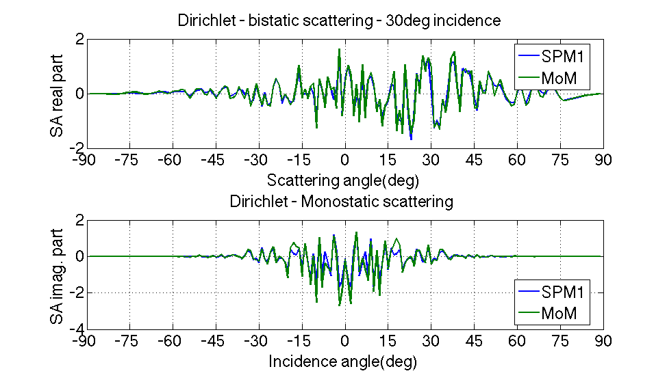
The Dirichlet boundary condition

Enforcing $\psi(x,\eta(x))=0$ on the surface leads to :

$B_0(k_0)=-q_0$
$B_1(k,k_0)=2iqq_0$
$B_2(k,x,k_0)=2qq_xq_0$ with $q_x=\sqrt{K_0^2-x^2}$

BD0=@(k0) -qf(k0,1);
BD1=@(k,k0) 2*1i*qf(k,1).*qf(k0,1);
BD2=@(k,x,k0) 2*qf(k,1).*qf(x,1).*qf(k0,1);
load('spm1Ddet.mat','momD') % the Method of Moments provides a numerical solution of the rigorous problem
figure(1)
subplot(211)
ii=find(tid==30);
H1=plot(tsd,real(spm(BD1,z,K0*sind(tsd),K0*sind(tid(ii)))),tsd,real(momD(:,ii)));
set(gca,'FontSize',24,'XLim',[-90 90],'XTick',[-90:15:90])
set(H1,'LineWidth',2)
grid on,xlabel('Scattering angle(deg)')
ylabel('SA real part')
legend('SPM1','MoM','Location','Best'),title(sprintf('Dirichlet - bistatic scattering - %ideg incidence',tid(ii)))
subplot(212)
H1=plot(tid,imag(spm(BD1,z,K0*sind(tsd),K0*sind(-tid))),tid,imag(diag(fliplr(momD))));
set(gca,'FontSize',24,'XLim',[-90 90],'XTick',[-90:15:90])
set(H1,'LineWidth',2)
grid on,xlabel('Incidence angle(deg)')
ylabel('SA imag. part')
legend('SPM1','MoM','Location','Best'),title(sprintf('Dirichlet - Monostatic scattering'))

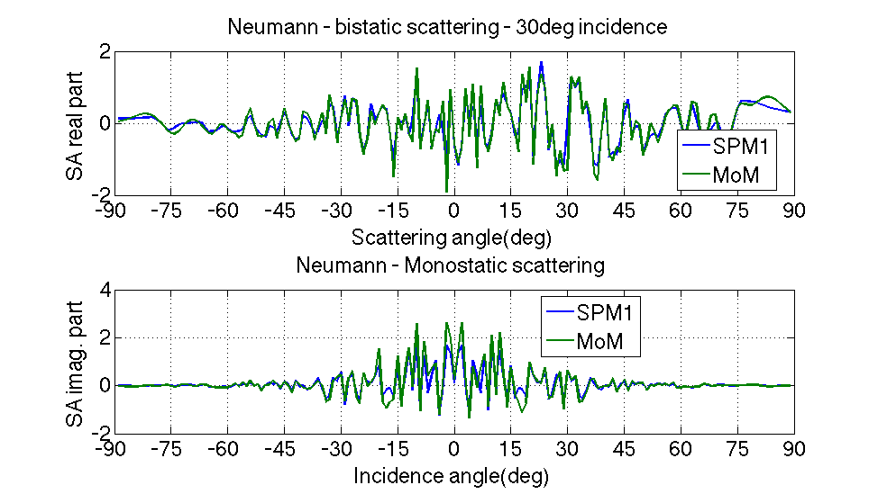
The Neumann boundary condition

Enforcing $(\mathbf{\hat n\cdot grad\,}\psi(x,\eta(x))=0$ on the surface leads to :

$B_0(k_0)=+q_0$
$B_1(k,k_0)=-2i(K_0^2-kk_0)$
$B_2(k,x,k_0)=-2(K_0^2-kx)(K_0^2-k_0x)/q_x$

BN0=@(k0) +qf(k0,1);
BN1=@(k,k0) -2*1i*(K0^2-k.*k0);
BN2=@(k,x,k0) -2*(K0^2-k.*x).*(K0^2-k0.*x)./qf(x,1);
load('spm1Ddet.mat','momN') % the Method of Moments provides a numerical solution of the rigorous problem
figure(2)
subplot(211)
ii=find(tid==30);
H1=plot(tsd,real(spm(BN1,z,K0*sind(tsd),K0*sind(tid(ii)))),tsd,real(momN(:,ii)));
set(gca,'FontSize',24,'XLim',[-90 90],'XTick',[-90:15:90])
set(H1,'LineWidth',2)
grid on,xlabel('Scattering angle(deg)')
ylabel('SA real part')
legend('SPM1','MoM','Location','Best'),title(sprintf('Neumann - bistatic scattering - %ideg incidence',tid(ii)))
subplot(212)
H1=plot(tid,imag(spm(BN1,z,K0*sind(tsd),K0*sind(-tid))),tid,imag(diag(fliplr(momN))));
set(gca,'FontSize',24,'XLim',[-90 90],'XTick',[-90:15:90])
set(H1,'LineWidth',2)
grid on,xlabel('Incidence angle(deg)')
ylabel('SA imag. part')
legend('SPM1','MoM','Location','Best'),title(sprintf('Neumann - Monostatic scattering'))

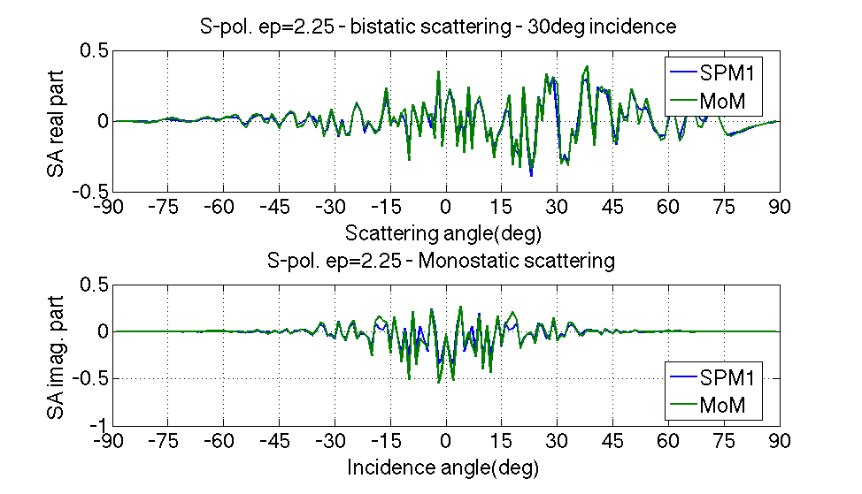
The transmission problem for S-polarized electromagnetic waves

With reflexion coefficient 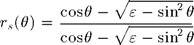$r_s(\theta)=\frac{\cos\theta-\sqrt{\varepsilon-\sin^2\theta}}{\cos\theta-\sqrt{\varepsilon-\sin^2\theta}}$ and associated transmission coefficient $t_s(\theta)=1+r_s(\theta)$ , the SPM coefficients write,

$B_0(k_0)=q_0r_s(\theta_i)$
$B_1(k,k_0)=iK_0^2\frac{\varepsilon-1}{2}t_s(\theta_d)t_s(\theta_i)$

rs=@(k,ep) (qf(k,1)-qf(k,ep))./(qf(k,1)+qf(k,ep));
ts=@(k,ep) 1+rs(k,ep);
BS0=@(k0,ep) +qf(k0,1).*rs(k0,ep);
BS1=@(k,k0,ep) 0.5*1i*K0^2*(ep-1).*ts(k,ep).*ts(k0,ep);
load('spm1Ddet.mat','momS','ep') % the Method of Moments provides a numerical solution of the rigorous problem
figure(3)
subplot(211)
ii=find(tid==30);
H1=plot(tsd,real(spm(@(k,k0)BS1(k,k0,ep),z,K0*sind(tsd),K0*sind(tid(ii)))),tsd,real(momS(:,ii)));
set(gca,'FontSize',24,'XLim',[-90 90],'XTick',[-90:15:90])
set(H1,'LineWidth',2)
grid on,xlabel('Scattering angle(deg)')
ylabel('SA real part')
legend('SPM1','MoM','Location','Best'),title(sprintf('S-pol. ep=%g - bistatic scattering - %ideg incidence',ep,tid(ii)))
subplot(212)
H1=plot(tid,imag(spm(@(k,k0)BS1(k,k0,ep),z,K0*sind(tsd),K0*sind(-tid))),tid,imag(diag(fliplr(momS))));
set(gca,'FontSize',24,'XLim',[-90 90],'XTick',[-90:15:90])
set(H1,'LineWidth',2)
grid on,xlabel('Incidence angle(deg)')
ylabel('SA imag. part')
legend('SPM1','MoM','Location','Best'),title(sprintf('S-pol. ep=%g - Monostatic scattering',ep))

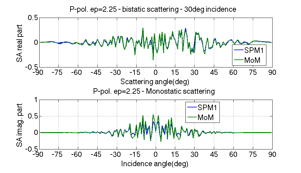
The transmission problem for P-polarized electromagnetic waves

Here, $r_p(\theta)=\frac{\varepsilon\cos\theta-\sqrt{\varepsilon-\sin^2\theta}}{\varepsilon\cos\theta-\sqrt{\varepsilon-\sin^2\theta}}$ and $t_p(\theta)=1+r_p(\theta)$ , so that

$B_0(k_0)=q_0r_p(\theta_i)$
$B_1(k,k_0)=i\frac{\varepsilon k k_0-\sqrt{K_0^2\varepsilon-k^2}\sqrt{K_0^2\varepsilon-k_0^2}}{\varepsilon^2}\frac{\varepsilon-1}{2}t_p(\theta_d)t_p(\theta_i)$

rp=@(k,ep) (ep*qf(k,1)-qf(k,ep))./(ep*qf(k,1)+qf(k,ep));
tp=@(k,ep) 1+rp(k,ep);
BP0=@(k0,ep) +qf(k0,1).*rp(k0,ep);
BP1=@(k,k0,ep) 0.5*1i*((ep-1)*(ep*k.*k0-qf(k,ep).*qf(k0,ep))/ep^2).*tp(k,ep).*tp(k0,ep);
load('spm1Ddet.mat','momP','ep') % the Method of Moments provides a numerical solution of the rigorous problem
figure(4)
subplot(211)
ii=find(tid==30);
H1=plot(tsd,real(spm(@(k,k0)BP1(k,k0,ep),z,K0*sind(tsd),K0*sind(tid(ii)))),tsd,real(momP(:,ii)));
set(gca,'FontSize',24,'XLim',[-90 90],'XTick',[-90:15:90])
set(H1,'LineWidth',2)
grid on,xlabel('Scattering angle(deg)')
ylabel('SA real part')
legend('SPM1','MoM','Location','Best'),title(sprintf('P-pol. ep=%g - bistatic scattering - %ideg incidence',ep,tid(ii)))
subplot(212)
H1=plot(tid,imag(spm(@(k,k0)BP1(k,k0,ep),z,K0*sind(tsd),K0*sind(-tid))),tid,imag(diag(fliplr(momP))));
set(gca,'FontSize',24,'XLim',[-90 90],'XTick',[-90:15:90])
set(H1,'LineWidth',2)
grid on,xlabel('Incidence angle(deg)')
ylabel('SA imag. part')
legend('SPM1','MoM','Location','Best'),title(sprintf('P-pol. ep=%g - Monostatic scattering',ep))